
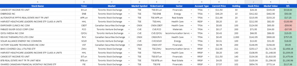
Part of any stock trader/investor’s job is to track their performance and profitability. There are many platforms to do this including your own brokerage accounts, yet sometimes this can be limited in terms of their features, functions and visualizations. In addition, this may be difficult for some investors and/or traders if they are using multiple brokerages and trading accounts as their portfolio are distributed and not all in one place. To aid with this I have created a simple Google Sheet that automatically looks up the current stock price using Google Finance API’s to automatically update your portfolio as shown below.
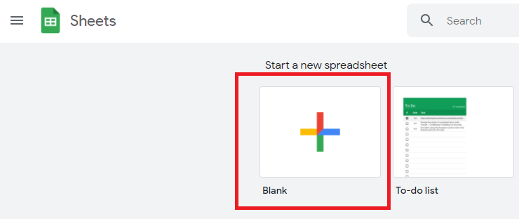
To do this first you need to create a new Google Sheet by opening https://sheets.google.com and click “Blank”.
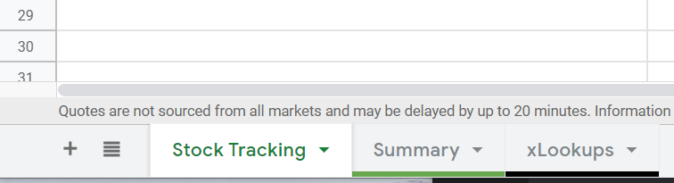
First add 2 additional tabs to the sheet by clicking the “+” button 2 additional time, then change the tab names by double clicking the tab at the bottom of the screen:
- Stock Tracking (Data Entry tab)
- Summary (Presentation Tab)
- xLookups (used to Data Validation and sheet Lookups)
Next, go to the Sheet “Stock Tracking” and create a header row with the following Column Headings:
- Stock Name (A)
- Ticker (B)
- Market (C)
- Market Symbol (D)
- TickerConCat (E)
- Sector (F)
- Account Type (G)
- Current Price (H)
- Holding (I)
- Book Price (J)
- Market Value (K)
- P/L (L)
We will go over each of these columns shortly including what these mean and what they do.
Copy the entire header row from the “Stock Tracking” tab to the “Summary” Tab, and add a “2” ad the end of each column name. For example on the “Stock Tracking” tab you will have a column called “Stock Name”, and on the “Summary” tab you will have the same column just named “Stock Name2”. Repeat this process for all columns in the “Summary Sheet”.
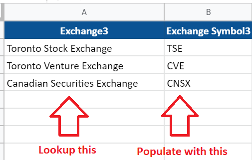
Next goto the “xLookups” Tab and enter the following. Please note that I am located in Canada, and this example is Canadian Focused but can easily be updated to address any market and account type.
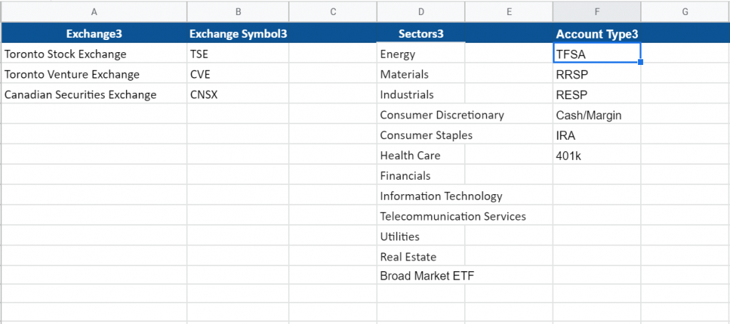
For the Exchange3 column and Exchange Symbol3 column you will need to find out the exchange symbols and convention for their lookups. You can do this by going to the google finance page and searching for your symbol as shown with the example for Apple.
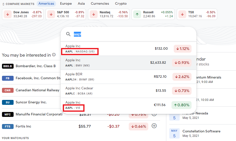
Here we see AAPL is traded on the NASDAQ and Google refers to this as NASDAQ when referencing the exchange, but also on the Vienna Stock Exchange using the Exchange symbol of VIE. Continue the process for each exchange you want to track stocks on and add the Exchange Name to column A of the “xLookups” tab, and the Exchange Symbol to column B of the “xLookups” tab.
Next, goto the “Summary” Tab, and in Cell “A2” add the following formula.
=FILTER(‘Stock Tracking’!A:AL, (‘Stock Tracking’!G:G=”TFSA”) + (‘Stock Tracking’!G:G=”RESP”)+ (‘Stock Tracking’!G:G=”RRSP”))

Please note the above example will only add TFSA, RESP and RRSP to the Summary tab. If you are using other account types you will need to adjust the formula to display these on this sheet. This is the tab that will be used to create visualizations, charts/graphs, and other fun stuff that will be addressed in further posts.
Next, goto the “Stock Tracking” Tab, and we will add the dropdown menus to the “Market”, “Sector”, and “Account Type” fields.
Market Lookup
For the “Market” Column lookup, select Cell “C2:C250” (this will add the lookups to row 250, if more are required) continue this for the necessary number of rows. Now right click in the selected columns and select the last option “Data Validation” and the following menu will pop-up.
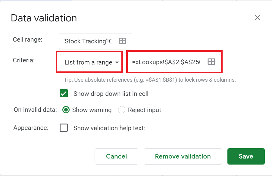
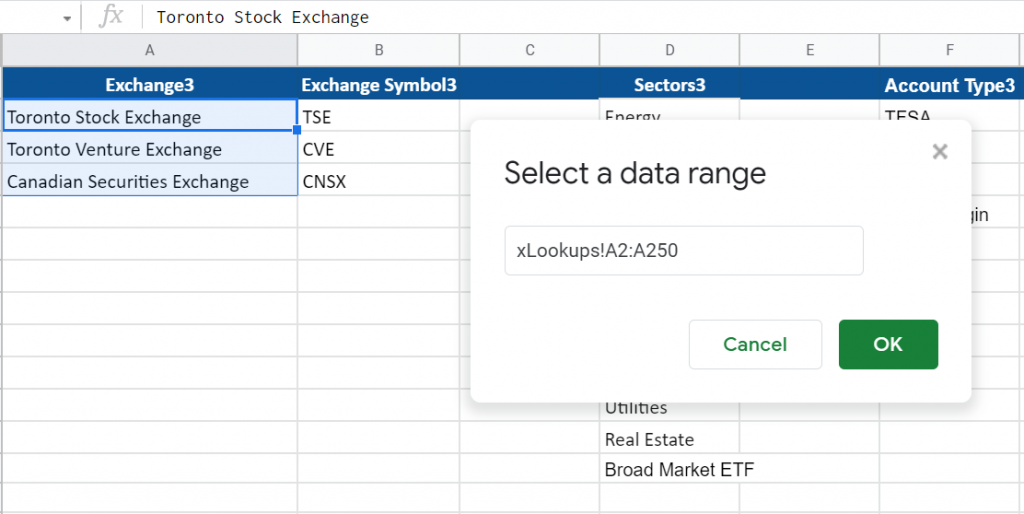
Change the “Criteria” option to “List from a Range”, and in the box beside “List from a Range” click the 4 squares at the end and it will prompt you to select the range. To do this goto the “xLookups” tab and select Cell A2:A250.
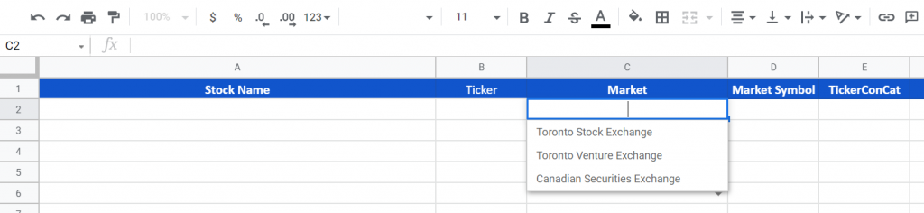
Click “Ok” then click “Save”, and now you will have a dropdown menu in the “Stock Tracking” Tab to select the exchange.
Sector Lookup
Next goto the “Sector” column (F) on the “Stock Tracking Sheet”, and select Cells f2:f250, and right click and select Data Validation again. Follow the same process as above and select Cells D2 to D13 on the “xLookups” tab. Click “Ok” and “Save” on the data validation window.
Account Type Lookup
For the “Account Type” column (G) repeat the above process again and select the “Account Types” from the “xLookups” tab in Column (F). Once the drop-down menus have been added you should see a down-arrow in the right corner of the cells that were updated, and you will be able to see your options.
Exchange Symbol vLookup
Next we need to add some formulas and calculations to get the ticker symbol and exchange in the correct format so Google Finance can do the current price lookup. To start in the “Market Symbol” column on the “Stock Tracking” Tab we want to do a VLookup on the “xLookups” sheets to find the proper Exchange symbol.
In the “Market Symbol” column of “Stock Tracking” Tab select cell D2 and enter the below formula.
=VLOOKUP(C2,xLookups!A2:B250,2,FALSE)
Continue this process by adding the the formula to all cells in the Market Symbol column to cell 250. Be careful when you do this as for example if you just drag the cell down to copy the formula you will be changing the the formula and incrementing the formula values by 1.
Moving on to cell D3 it should have the following formula.
=VLOOKUP(C3,xLookups!A2:B250,2,FALSE)
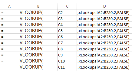
The only thing that should be changing in this formula is the first parameter in the vlookup formula, “C2”, and in the following row it should be C3, then C4, etc…. This can be tricky to do and keep the formula’s correct and in order. I typically use excel to do this which takes a few extra steps but is alot easier then manually entering the changing formulas.
To do this split the formula up and essentially have the value that changes in its own column. For the cells that just need to repeat down without changing (A, B & D), use copy and paste to fill these down to row 250. For column “C” in this example, select the cell and drag it down to row 250. This will change the value from C2 to C3, to C4, etc….
Next copy all data as is, and paste it into notepad and it should like similar to the below.
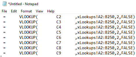
Use search and replace to remove the tab, and unnecessary spaces, and once completed to back to your Google Sheet and select cell D2 and paste the copied formulas from Notepad. This will paste the proper formulas into all cells.
TickerConCat
The next column we will work on is the “TickerConCat” which simply just takes the stock ticker symbol, and the market exchange and concatenates them into a format that can be used to query Google Finance. To do this is fairly simple and just add the following formula into cell “E2”.
=CONCATENATE(D2,”:”,B2)
Once this has been done, drag the small square in the bottom right corner of the cell down to row 250. This will updates the values within the formula as you go down the rows.
Google Finance Query
Now we can add the Google Finance Lookup for the stock Symbol. To do this select cell H2 and enter the following formula.
=GOOGLEFINANCE(E2)
Once this has been done, drag the small square in the bottom right corner of the cell down to row 250. This will updates the values within the formula as you go down the rows.
Market Value
Now we can calculate the Market Value of the holdings by adding a simple formula in the K2 field which is simply multiplying columns “I” (current position size) and column “H” (Current Price)
=H2*I2
Once this has been done, drag the small square in the bottom right corner of the cell down to row 250. This will updates the values within the formula as you go down the rows.
Profit and Loss Calculation
To calculate the Profit and Loss simply add the following formula which calculates the difference between Book Value and Market value columns.
=K2-J2
Once this has been done, drag the small square in the bottom right corner of the cell down to row 250. This will updates the values within the formula as you go down the rows.
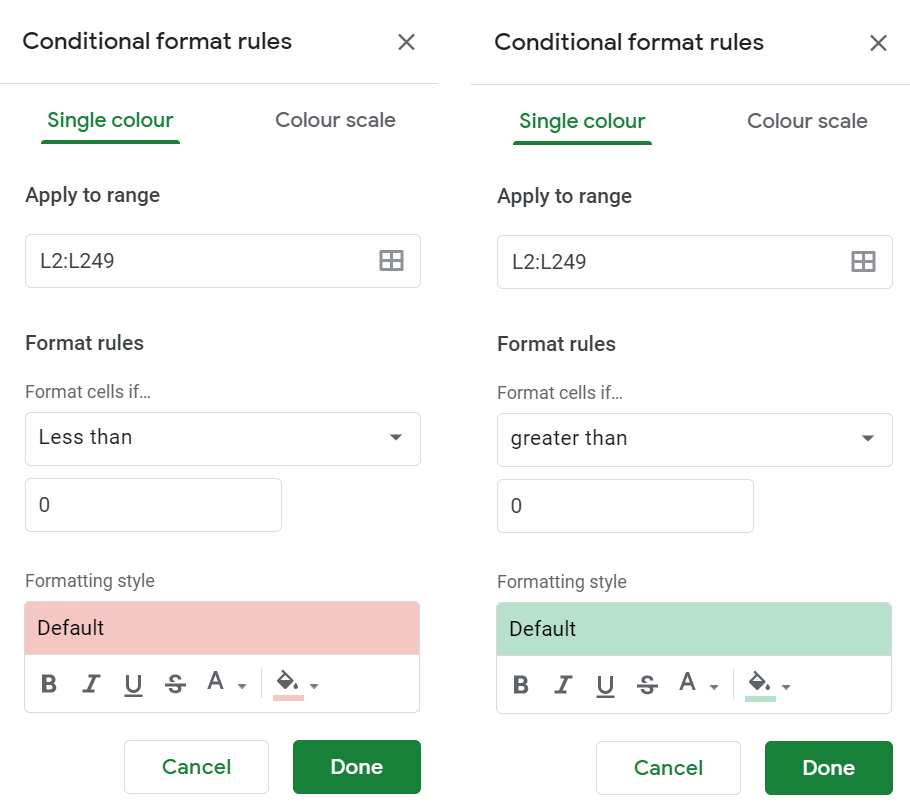
Next select cells L2 -> L250 and right click and select conditional formatting. This will change the colour of the cells red or green depending on profit or loss. To do this add a condition where if the value in this cell is above “0” make the cell green, and add a second condition for if the value is below “0” it will be red.
Now the Fun Part
In the “Stock Tracking” start to enter your portfolio information in the cells and watch the data update as you go.

As you continue to enter the data is will populate and do its calculations. If you wish to do any charts / graphs / or other visualizations you will need to do this off the “Summary” tab as the “#N/A” cells and drop-downs with no values will mess up the visualizations.
Visualizations and other fancy things you can do with this now will be described in a following blog post.